Socceconomics: A simple, well-calibrated model for expected goals

It was about time to expand the reach of this blog to other sports than basketball and American football and we did. Alex Fairchild, Marios Kokkodis and myself got to explore what makes a shot in (rest-of-the-world football or else) soccer successful, i.e., end up at the back of the net.  This is the notion of expected goals, which has been around for quiet a while now in the radar of soccer practitioners and there are several models that have appeared.  In our work we are more focused on the evaluation of such models and on the implications for evaluating players and teams.  This post is a condensed version of our forthcoming paper in the Journal of Sports Analytics, entitled “Spatial Analysis of Shots in MLS: A Model for Expected Goals and Fractal Dimensionality”.

Alex compiled a set of 1,115 (non-penalty) shots from 99 MLS games during the 2016 regular season between March 6 – May 18, 2016. The John Burn-Murdoch’s soccer pitch tracker was used to tag each shot’s location, outcome, game state, assist type, and to define the phase of play from which the shot came (i.e. set piece, open play, etc.).  Using this dataset we built a simple logistic regression model for the probability of a shot ending up to a goal given a set of shot features.  The following spatial density plots depict the positive (goals) and negative (non-goals) class of our model. 

The features we used for training our regression model are:

• Location information: This includes the coordinates (x,y) of the location that the shot took place from
• Distance: This is the distance of the shot location from the goal line
• Shot angle: This is the angle created by the two straight lines connecting the shot location with each of the vertical goal posts
• Shot type: This is a categorical variable that captures whether the shot was a header, a right or left leg shot.
• Assist type: This is a categorical variable that captures the type of assist that resulted to the shot
• Play type: This is a categorical variable that describes whether the play was a set piece or an open play.

 The following table presents the results, where as we can see, really the shot distance and shot angle are the most important factors as one might have expected.  Of course, our model does not account for important contextual features such as the number of defenders around the ball at the time of the shot, the closest defender etc.

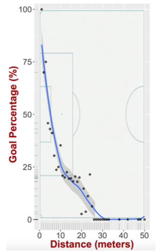
For example, all else being equal, the probability of scoring a goal declines with the distance from the goal line as seen in the following figure.

However, one could argue all of these are well-known and common knowledge.  How well does it predict whether a shot ended up in a goal or not? However, with a second thought is this really the right question? Is accuracy in predicting goals what soccer practitioners should be after for this type of models? Our answer to this is of course no! Imagine the case that you have two models M and M’ assign to a shot a probability 0.1 and 0.4 respectively for scoring.  These two models will exhibit exactly the same accuracy, since in essence they both predict that the shot will not end up in a goal (assuming the typical probability threshold of 0.5). However, if one was to use these two models to evaluate a player and the decisions he makes with regards to the shots he takes, the conclusions would be completely different! Based on model M the player that took this shot did not judge very well since he took a shot with very long odds of ending up in a goal.  So the right question is how accurate is the probability outcome of the logistic regression model (or any expected goals model).

Ideally we would like the exact same shot to be taken 100 times, measure how many times ended up in a goal and then compare with the probability given by the model.  However, this is clearly not possible and hence, we will use all the shots in our dataset.  We can group the shots based on their predicted probability and then we can see for every group which fraction of the shots ended up in a goal.  Ideally we would like the corresponding line to be as close as possible to the y=x line, since this means that the probability we get from our model is consistent with what happens in reality. For our results we used probability bins of 10% and we got the following results:

As we can see the line is statistically not different than the y=x line (95% confidence interval for the slope [0.77,1.1] and for the intercept [-0.01,0.04]).  Using this probability model we then model the expected number of goals from a sequence of shots (either player shots or team shots) through a Poisson binomial distribution, which is the sum of independent (but not necessarily identically distributed) Bernoulli trials.  Using that the expected number of goals for team T, taking shots St is given by:

Comparing the actual number of goals a team scored (allowed) and the expected number of goals we can get their offensive (defensive) efficiency:

where G(T,+) (G(T,-)) is the number of goals scored (allowed) by the team. Using these team efficiencies we can then classify the teams based on where they fall on the 2D plane of the efficiencies:

Finally, we touched upon the reasons that drive teams’ efficiencies and we focused on the spatial analysis of the locations of their shots. We wanted to describe the distribution of the shots with a single number and for this we used the notion of fractal dimension that we have used several times in the past (here, here and here). Our findings indicate that the teams that exhibit higher fractal dimension have lower offensive efficiency (correlation was moderate -0.36).  This might seem counter intuitive, since one might expect that taking shots from a variety of locations would stretch the defense more, create more open spaces and hence, create better situations for scoring. However, the opposite is true and one of the reasons might be the fact that a team by having its shots uniformly distributed over the space, will end up taking many low quality shots. Furthermore, the defenses are aware of the low chance of making a shot from a long distance and hence, the stretching of the defense is less than expected.

More details can be found in our full paper. This is just the beginning for the endless possibilities of an expected goals model.  However, we first need to make sure the model captures what it is supposed to (i.e., the actual goal probability).