In-game win probabilities Part 2: iWinrNFL

In the first part of our dealing with in-game probabilities we made some general comments about issues (or not) with these models. One of the problems with existing models is that they are not open, i.e., very little is known about their mechanics. Here I will present the details and the evaluation of a simple, yet well-calibrated win-probability model, which we call iWinrNFL (short for “in-game Winner NFL”).  More details about the model can be found in the technical report.

The problem of in-game win probability is to identify the chances of a team (e.g., the home-team without loss of generality) winning the game given the current state of the game.  One of the first decisions to be made is how one describes the current state of the game, or simply put what are the features of the model. For iWinrNFL the following are the features used:

1. Ball Possession Team: This binary feature captures whether the home or the visiting team has the ball possession

2. Score Differential: This feature captures the current score differential (home – visiting)

3. Timeouts Remaining: This feature is represented by two independent variables – one for the home and one for the away team – and they capture the number of timeouts remaining for each of the teams

4. Time Elapsed: This feature captures the time elapsed since the beginning of the game

5. Down: This feature represents the down of the team in possession

6. Field Position: This feature captures the distance covered by the team in possession from their own yard line

7.Yards-to-go: This variables represents the number of yards needed for a first down

8. Ball Possession Time: This variable captures the time that the offensive unit of the home team is on the field

9. Ranking Differential: This variable represents the difference of the win percentage for the two team (home – visiting)

The model itself is based on a logistic regression model.  While for a game of infinite duration a linear model could be a very good approximation, the finite duration of the game creates non-linearities, especially towards the end of the game.  For this reason, we use a logistic regression model for the first 57 minutes of the game, and a support vector machine model (with radial kernel) for the last 3 minutes of the game (the choice of the 57-3 is arbitrary, but it can be evaluated if one wants). The raw output of the support vector machine classifier is not a probability and hence, we use Platt’s scaling for obtaining a class probability. In a nutshell iWinrNFL is depicted in the following:

In order to train the model I collected all the play-by-play data from the past 8 regular seasons and extracted the featured needed.  I interacted directly with the NFL API but there is an easier solution to use the nflscrapr library developed by the folks at the CMU sports analytics student club. This provided 2,048 regular season games and 338,294 snaps. The way to set up the training is to get every play and for each one of the plays to extract the state of the game, i.e., the corresponding features.  Then the dependent variable for this instance will be 1 if the home team won the game eventually and 0 otherwise. I have also included in the model three interaction terms between the ball possession team variable and (i) the down count, (ii) the yards-to-go, and (iii) the field position variables. This is crucial in order to capture the correlation between these variables and the probability of the home team winning. The interpretation of these variables is different depending on whether the home or visiting team have the ball possession. These interaction terms will allow the model to better distinguish between the two cases. The logistic regression standardized coefficients are shown in the following table.

As we can see, as one might have expected the current scoring differential exhibits the strongest correlation with the in-game win probability. The only factors that do not appear to be statistically significant predictors of the dependent variable are the down and the yards-to-go. Even though the corresponding coefficients are negative as one might have expected (e.g., being at an earlier down gives you more chances to advance the ball), they are not significant in estimating the win probability. On the contrary, all else being equal timeouts appear to be quiet important since they can help a team stop the clock, while teams with better win percentage appear to have an advantage as well, since this can be a sign of a better team.

We then evaluated the calibration of iWinrNFL through the reliability diagram. In particular, we grouped instances in our test set (split 70-30) at bins of 0.05 probability.  Our results are presented in the following figure.

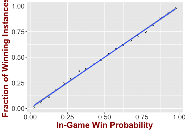
As we can see the predicted probabilities match very well with the actual outcome of these instances. The fitted line has a slope of 0.993 (with a 95% confidence interval of [0.98,1.01]), while the intercept is 0.0047 (with a 95% confidence interval [-0.006, 0.012]), while the R-squared is 0.99. Simply put the line is for all practical purposes the y=x line, which translates to a fairly consistent and accurate win probability.  Also, with the typical decision boundary of 0.5 probability, the accuracy of iWinrNFL is 75%. More evaluation results can be found in the technical report.

Finally, we applied our model at this year’s Super Bowl. Super Bowl 51 has been labeled as the biggest comeback in the history of Super Bowl. Late in the third quarter New England  Patriots were trailing by 25 points and Pro Football Reference was giving Patriots a 1:1000 chance of winning the Super Bowl, while ESPN a 1:500 chance.  PFR considers this comeback a once in a millennium comeback. While this can still be the case as alluded to above, in retrospect Patriots’ win highlights that these models might be too optimistic and confident to the team ahead. On the contrary, the lowest probability during the game assigned to the Patriots by iWinrNFL for winning the Super Bowl was 2.1% or about 1:50. We would like to emphasize here that the above does not mean that iWinrNFL is “better” than other win probability models. However, it is a simple, open model that assigns win probabilities in a conservative (i.e., avoids “over-reacting”), yet accurate and well-calibrated way.

A shiny app implementing this model can be found here (if the app is temporarily unavailable, excuse me but I have the free shinny version 🙂 – following is a screenshot on how it looks).