Skill Curves in the NFL: Unlocking the Interactions between Passing & Rushing

The NFL has clearly turned to a pass-first league during the past decade or so, and for a good reason.  Passing is overall more efficient!  Indeed using play-by-play data from the 2014-2016 NFL seasons and the Winston-Sagarin-Cabot model for expected points, a passing play adds on average 0.25 expected points, while a rushing play adds on average only 0.06 points. This has led many people to condemn teams that still exercise a run-heavy game. In this work we revisit the importance (or not) of the rushing game, by examing the passing skill curve in NFL.  In particular, borrowing from Dean Oliver’s seminal work on basketball analytics we explore the efficiency of a passing play as a function of its utilization.  Dean Oliver identified that the efficiency of a basketball player (e.g., true shooting) declines with an increase of his utilization (e.g., fraction of total team shots taken by him).  Hence, the central hypothesis in this work is that passing efficiency exhibits a similar skill curve, which consequently means that we cannot blindly increase the number of passing plays and expect the same efficiency.

In order to explore our hypothesis we used play-by-play data from the 2014-2016 NFL seasons.  In particular, for every game in our dataset we calculated for each team the utilization of passing as the fraction of passing plays over the total number of its offensive snaps. We further calculated the average expected points added for the passing plays for each team and each game.  We have adjusted the expected points for strength of defense.  The following figure presents the results (binned for better visualization), where to reiterate passing efficiency is the expected points added per passing play.  As we can see there is a declining trend for the passing efficiency as we increase its utilization.

The correlation coefficient is .  These results, while they account for quality of passing defense, they do not account for the quality of the rushing game as well as the overall passing ability of the team that can impact the results.  Therefore, we build a regression model where the independent variable is the average expected points added per passing play (adjusted for defense) within a game, while the dependent variables include:

• Passing utilization .
• Passing rating of the offense . This captures the performance expectations of the passing offense.
• Average expected points added per rushing play during the game under consideration. This captures how well the ground game has performed during the game under consideration.
• An interaction term between and .

The table above presents our results where we can see that the utilization is still negatively correlated with the expected points added per passing play.  The interaction term also shows that this correlation depends on the rushing ability of the offense.  In particular, the effect of passing utilization on its efficiency is , namely, if the offense runs the ball better the negative relationship between and is less strong.  In particular, with (the maximum observed value in our dataset), the corresponding coefficient is -0.42 — compared with a coefficient of -1.33 for the minimum value of in our dataset, i.e., -0.73.

So how much should a team run?  Obviously the question depends on many factors but it should be evident that calling passing plays all the time is going to have diminishing returns.  While the passing efficiency might still be greater than that of rushing even when , this does not mean that it is the best the team can do. What we a team is interested is maximizing the efficiency on a per-play basis regardless of the type of play, i.e.,

The following figure presents the passing utilization that maximizes the above equation for different values of and .  As one might have expected for teams with better passing rating a higher utilization is recommended for fixed rushing ability, while better running game reduces the optimal passing utilization.  Note that a rushing EPA higher than 0.3 per play per game is rather unrealistic, and so is having .  For the average rushing EPA (marked with the vertical line), the optimal fraction of passing plays is 0.3, 0.47 and 0.63, for a bad, average and great passing offense respectively.

I’d like to note here that the results of the analysis are not and should not be treated as causal, that is, running more does not necessarily cause passing to be more efficient.  It might as well be the case that teams that are trailing in the score turn to more passing and this bias the results. However, by estimating the league passing skill curve  at the end of third quarter (to avoid the artificial decrease of passing utilization from a team that is ahead), we still got a decreasing function:

When controling for quality of passing and rushing, utilization is still negatively corrlated with passing efficiency. Furtherore, we have estimated these curves using a different EPA model (in fact, the presence of many different EPA models might be one of the reasons that these models/statistics are still not mainstream). In particular, we used the EPA model used in nflWAR and is available at the nflscrapR package. Again similar results are obtained (slightly lower correlation).

Finally, we have treated rushing as being constant regardless of its utilization.  While rushing skill curves are weaker as compared to passing the final results will quantitatively (not qualitatively) change. However, it should be evident that there is a clear interaction between passing efficiency and utilization that makes rushing still a piece of the puzzle in the NFL.

Updated content [10/18/2018]

Various comments I got on the original version of this article were related to the importance of score differential in the game plan. The idea is that score differential will lead teams to pass more or less (depending on whether they are trailing or not) and thus, score differential needs to be accounted for. Overall I agree – especially in the case where a team jumped to an early lead through possibly efficient passing and then they turned to milking the clock, artificially reducing the pass utilization. I have mentioned this myself in the original article. However, I do not necessarily agree with the idea that if a team trails and starts passing more this skews the results. Utilization is utilization; it does not matter whether it was part of the game plan or part of in-game adjustment (in my opinion). Also some of the comments mentioned that teams that fall behind are typically bad teams and hence, they are expected to have low passing efficiency. Agreed (to an extend, maybe a small extend, but I agree overall). The good thing is we can control for all of these in a regression. And in fact some of them were in the original regression. The main thing that was not there and I will include now is a variable that captures the impact of score differential. Given that the score changes throughout the game I decided to use as a proxy the smallest score differential for a team through the game. Hence, if a team never trailed this will be 0, while if a team trailed this will be negative. I also added an additional interaction term between utilization and overal passing ability just for symmetry. Following are the results using data from nflscrapR (seasons 2014-2017):

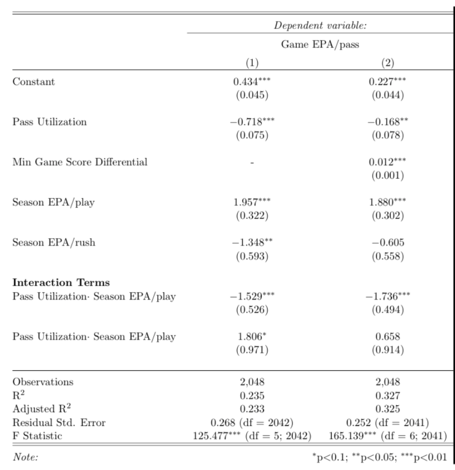
The first model does not include the score differential-related regressor, while we have added it in the second one. Despite the addition of this variable the utilization is still negatively correlated with the with the (game) passing efficiency. However, the strength of this relation is reduced – which is in agreement with the previous regression results when we had focused only on Q1-Q3. However, the season EPA/rush (and the corresponding interaction term) are not significantly correlated  anymore with the passing efficiency. This could be due to the fact that the score differential might drive more the efficiency (or lack of efficiency) of a team in a game through play-calling etc. Also of course, this regression only captures correlations, so it can also be that the pass efficiency is stronger correlated with score differential (good passing teams will have better chances to having a larger score differential) compared to the correlation between the rushing and passing game of a team. In any case, even adding the variable to capture score differential the passing volume (utilization) is still negatively correlated with the efficiency of the passing game. I will keep udpating this analysis either with other variables in the regression that I will think or you will suggest to me or with new methods (an econometrics approach is coming…).

Updated content [8/7/2018]

One of the questions that I keep getting is since running is so much less efficient how can one support (average) teams run as much as the optimization gives you (i.e., close to 50%)? Well I guess people don’t believe in optimization. But regardless, of course the above optimization is a crude reduction of a complex decision/problem, and the exact/true solution most probably is something else. Furthermore, the results presented above use the curves from the whole game, which might be impacted from the various biases mentioned above. If we used the curves from the end of Q3, the actual solutions would be different and a higher percentage of passes would be provided as a solution.  However, it should be clear that is not 100% passing, or heck not even 80% passing. Anyway, since I got asked a lot I will be updating this thread with testable hypotheses on why and when a team might be better off running more. In fact, the above analysis only tells us that there is an interaction between rushing and passing, but nothing about the reasons and mechanisms behind it. So let’s start.

A. The Anatomy of an Underdog’s Win

I have been thinking about underdogs a lot — who does not like it when an underdog wins. So one of the first things I want to examine is whether there is a benefit to rushing when you are playing a better team. There are many reasons that I can think of why this might be a true/plausible hypothesis, but the general idea is that more running reduces the pace and creates more variance for the outcome, similar to basketball even though clearly the number of possessions/drives is much smaller.  Anyway the reason why I think this might be a plausible hypothesis is not important; what is important is what the numbers say!

I collected Vegas betting lines for the 2009-2015 seasons and for every game with a more than 3 points underdog (to avoid fairly equally matched games)  I calculated the rushing fraction for the underdog and whether the dog won or not. Then I grouped the games based on the rushing utilization. For every group I calculated the expected number of underdog wins using the Vegas point spread. In particular, if a team is favored by points, the probability of this team winning the game is:

where, is the cumulative distribution function for the standard normal random variable. Then the expected number of games won by an underdog (p < 0) in a set of games is:

By comparing the actual games won by an underdog and the expected number won we get the following results:

As we can see a higher rushing rate for underdogs lead to more wins than expected. And because I know you are going to ask for reverse causality, all play fractions are calculated up to the end of Q3 in order to avoid “teams that have gone ahead in the score from passing, run the clock in Q4”.  OK this tells that more running from underdogs is associated with winning more than expected. But we still do not know why. People have pushed back on my initial reasoning saying that running more does not prolong the drives – i.e., reducing the pace. While this might be the case,  the evidence I have seen online (pointed to me by the critiques) are not compelling in the sense that what I see is basically a bunch of drives with 40% rushing plays that are anywhere between 5 and 20 plays. OK, this only tells us that a drive with 40% rushing will give you 5 to 20 plays in total. We still do not know what is the trend when rushing is 50% or 20%. We might still get the same variance (5 to 20) or we might get the same variance shifted (e.g., 10-30). Anyway, let’s assume that indeed running more does not decrease the total number of drives significantly – which to repeat it is highly plausible particularly given the low number of possessions to begin with. What else can be driving the result above? One of the potential reasons might be a lower number of TOs. TOs can happen both in rushing and passing so we obviously have to consider both of them. So let’s examine the TOs per game and their relation with rushing utilization. First we make the observation that the number TOs per game/per team follows a Poisson distribution. In particular, following is the number of TOs per game for underdogs – again Q1-Q3 so do not bring up the fact that a team that is behind the score will call more risky plays at Q4 – (the league-average is very similar — shifted to the left):

We have also plotted a Poisson distribution with mean 1.65 and as we can see they match fairly well. In fact, the chi-square test cannot reject the hypothesis that the true distribution of the data is a Poisson. Given that the TOs/team/game follows a Poisson distribution we run a Poisson regression for the number of TOs committed by an underdog during a game using as covariate the rushing utilization. We also do the same for the league-average case, i.e., not only considering underdogs. The following plot provides the expected number of turnovers obtained from the Poisson regression for underdogs and for the league.

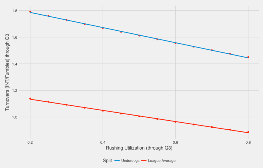
It is clear that overall underdogs commit more TOs on average (they are underdogs for a reason), but the mean of the Poisson distribution reduces with rushing utilization (I guess underdogs tend to have worse QBs…). Now for the league too, the relation is negative, but the slope observed is less steep (actually if we consider only the favorites the slope is very slow).  This basically means that underdogs will increase their TOs faster than favorites when they increase their passing rate. How much is this worth in terms of (expected) points? Using the expected points added for every play that led to a TO, a TO is worth approximately 4 points. Hence, when the TO rate is , the expected points lost from TO are:

Using this equation underdogs can “save” anywhere between 1.5-2 points per game from turnovers by running a little more. Obviously this does not explain the whole line they cover, but I would not expect there to be a single mechanism that explains the interaction between rushing and passing. Also when I mention that underdogs do not have good QBs I always get the response that well they do not have good RBs too. That’s most probably true, but it seems it is easier to throw and interception than fumble (?). Also if we break down the TOs, the expected points added for an INT is -4.7 on average, while for a fumble is -2.6 on average (possibly because more INT are returned for a TD – 11% of INT are pick-6s, while 5% of fumbles are returned for a TD).

In conclusion, it seems that there are supporting evidence for an underdog to run a little more. Again everything is observational but the evidence for this hypothesis seem compelling.